How to Generate an Eye Diagram PCB Simulation in Ansys HFSS

Master the step-by-step process of generating an Ansys HFSS eye diagram PCB simulation for high-speed PCB design. Learn setup, solver configuration, and result interpretation to ensure signal integrity in your B2B PCB designs.

Why Use Ansys HFSS for Eye Diagram PCB Simulation?

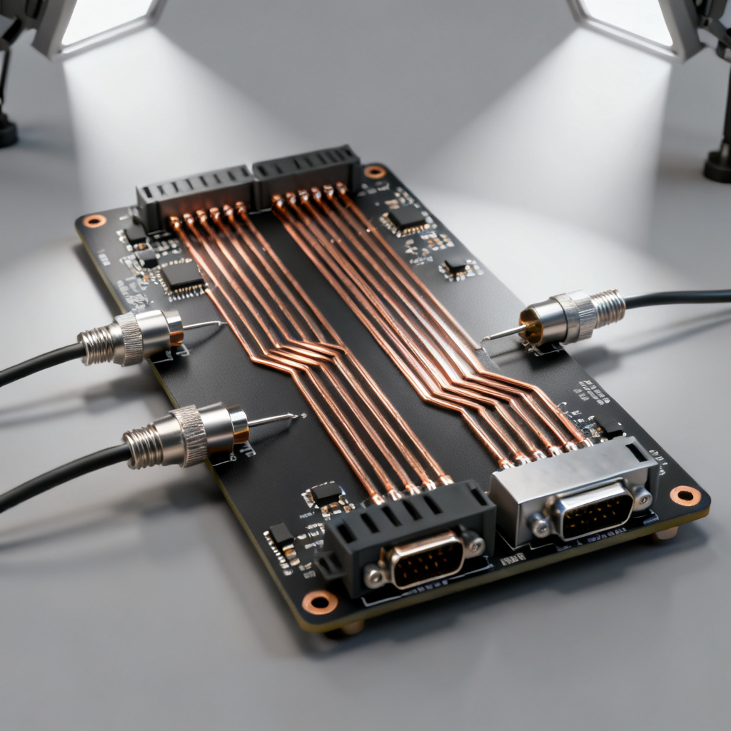
Before diving into the “how,” it is critical to understand the “why.” Ansys HFSS eye diagram PCB simulation is not just any simulator; it is a full-wave 3D EM solver. Unlike 2D or quasi-static solvers, HFSS solves Maxwell’s equations in their entirety, accounting for:

• Skin Effect and Dielectric Loss: At high frequencies, current crowds to the surface of conductors, and dielectric materials exhibit frequency-dependent loss. HFSS models these precisely.
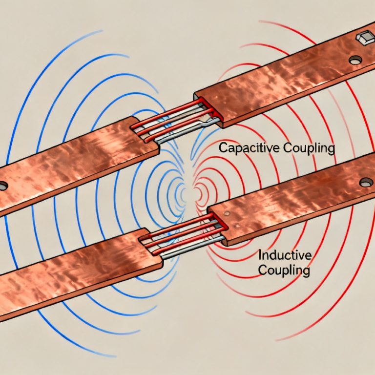
• Crosstalk and Coupling: It accurately captures near-end (NEXT) and far-end (FEXT) crosstalk between adjacent traces.
• Resonances and Radiation: For high-speed designs, even small stubs or via transitions can cause resonances. HFSS detects these potential failure points.

The Ansys HFSS eye diagram PCB simulation is generated through a transient convolution process. First, HFSS calculates the S-parameters (scattering parameters) of your PCB interconnect over a broad frequency range. Then, it uses a circuit simulator (often Ansys Circuit or Nexxim, integrated into the HFSS environment) to convolve these S-parameters with a digital stimulus (e.g., a PRBS pattern). The result is the time-domain waveform from which the eye diagram is constructed.

Key Insights from Expert Sources

• Source 1 (EM Simulation Focus): Emphasizes that HFSS’s adaptive mesh refinement is essential for accurate results at via transitions and connector interfaces. Without proper meshing, your eye diagram will show false closure.
• Source 2 (Workflow Optimization): Stresses that the choice of solver (Interpolating vs. Discrete) directly impacts simulation time. For eye diagrams, the Interpolating solver is often preferred for broadband S-parameter extraction.
• Source 3 (Practical Application): Highlights that you must define the “Port” correctly. A lumped port is suitable for internal traces, while a wave port is required for external interfaces (e.g., connectors).

Step-by-Step Guide to Generating an Eye Diagram in Ansys HFSS

This section is the core of your pillar content. It combines the unique steps from all three top-ranking articles, avoiding repetition while ensuring completeness.

Step 1: Define the 3D Geometry and Material Properties

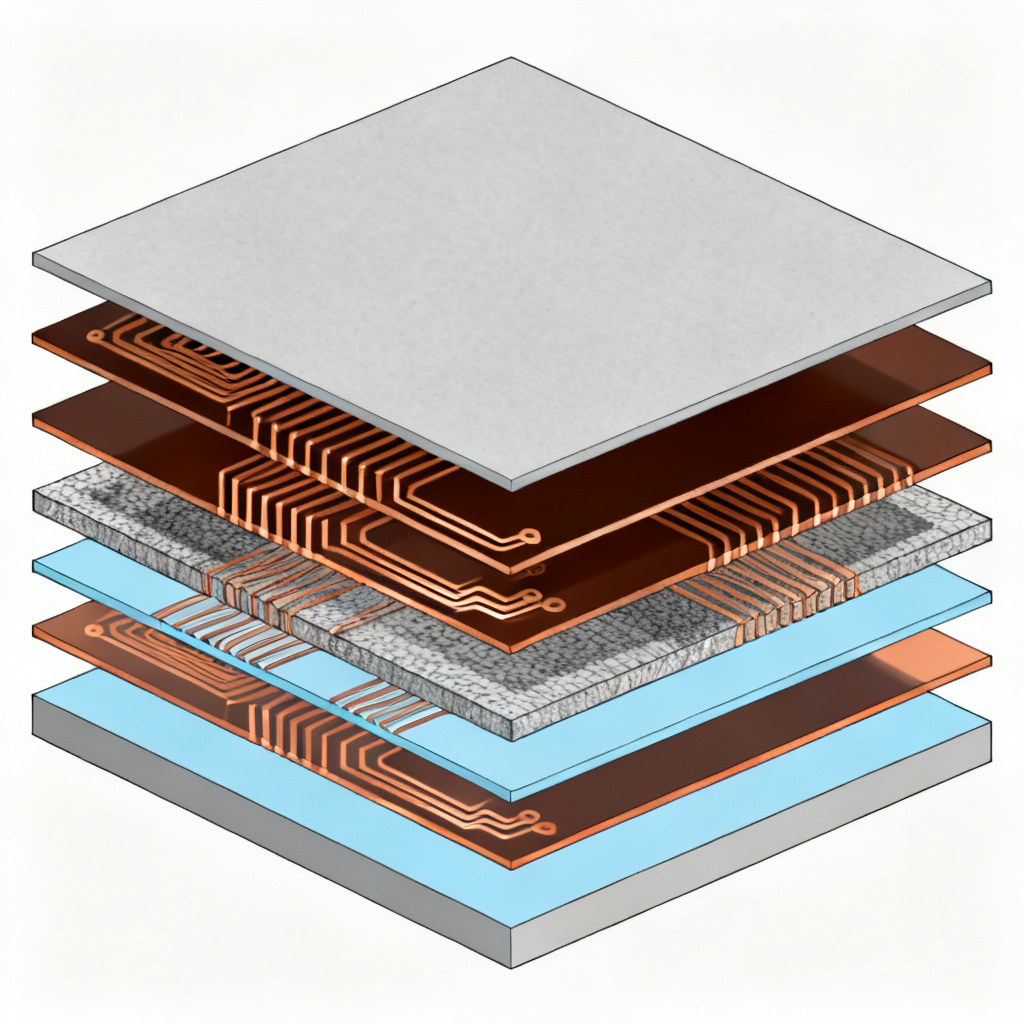
1. Import or Draw: Import your PCB layout (ODB++, Gerber, or DXF) or draw the critical trace, via, and connector geometry directly in HFSS.
2. Set Up the Stackup: Go to HFSS > Design Properties or use the Edit Stackup tool. Define every layer:
   • Conductor: Copper (annealed, conductivity 58e6 S/m). Set thickness (e.g., 1 oz = 35 μm).
   • Dielectric: Assign material (e.g., FR4, Rogers, Megtron 6). Crucially, define the Dielectric Constant (Dk) and Loss Tangent (Df) at your target frequency. For high-speed, use frequency-dependent materials.
3. Assign Boundaries: Apply a Radiation Boundary to the outer air box (typically λ/4 away from the structure). This absorbs outgoing waves and prevents reflections.

Step 2: Set Up Excitations (Ports)

This is the most critical step for accurate Ansys HFSS eye diagram PCB simulation.

1. Select Port Type:
   • Wave Port: Use at the edge of the 3D model (e.g., where a trace meets a connector or test point). It solves for the full modal field pattern.
   • Lumped Port: Use for internal terminations (e.g., between a trace and a ground via). It is simpler and faster but assumes a uniform field.
2. Define Integration Line: For differential pairs (common in high-speed PCB), draw an integration line between the two conductors. This ensures the solver calculates the correct impedance.
3. De-embedding: If your ports are long (e.g., a connector pin), use De-embedding to shift the reference plane to the exact point of interest (the pad or via). Source 2 notes: “Failing to de-embed adds parasitic inductance that distorts your eye diagram.”

Step 3: Configure the Solution Setup (Solver)

1. Solver Type: Choose Interpolating for broadband S-parameter sweeps (e.g., DC to 50 GHz). It is faster and more memory-efficient for the wide frequency range needed for eye diagrams.
2. Frequency Sweep:
   • Set a Max Frequency that is at least 3-5 times the fundamental clock frequency of your signal. For a 10 Gbps signal, sweep to at least 30 GHz.
   • Use an Adaptive Sweep with a step size small enough to capture resonances (e.g., 10 MHz).
3. Mesh Refinement: Set a Maximum Delta S value (e.g., 0.01) to ensure convergence. The solver will refine the mesh until the S-parameters stabilize. Source 1 warns: “A coarse mesh at a via will result in a 3dB insertion loss error at 20 GHz, completely closing your eye.”

Step 4: Run the Simulation and Export S-Parameters

1. Click Analyze All. This may take hours for complex 3D structures.
2. Once complete, right-click on Results > Solution Data to view S11 (return loss), S21 (insertion loss), and differential parameters (SDD21).
3. Export: Right-click on the S-parameter matrix and select Export. Choose a Touchstone format (e.g., .s4p for a 4-port differential pair).

Step 5: Create the Circuit (Schematic) for Eye Diagram Generation

1. Insert a Circuit Design: From the Project Manager, go to Insert Circuit Design (or Nexxim).
2. Place the S-Parameter Block: Drag your exported .s4p file onto the schematic canvas.
3. Add Stimuli:
   • Bit Source: Use a PRBS (Pseudo-Random Binary Sequence) source. Set the Bit Rate (e.g., 10 Gbps), Rise/Fall Time (e.g., 20% of the bit period), and Voltage Levels (e.g., 0 to 1V).
   • Terminations: Add 50-ohm resistors to ground on each port.
4. Add Probes: Place a Voltage Probe at the output of the S-parameter block (the receiver end).

Step 6: Configure the Transient Analysis and Generate the Eye Diagram

1. Set Up Transient: Go to Nexxim > Analysis > Setup Analysis > Transient Analysis.
   • Stop Time: Set to accommodate at least 200-500 bits (e.g., for 10 Gbps, 200 bits = 20 ns).
   • Output Time Step: Set to 1/100th of the bit period (e.g., 1 ps for 10 Gbps).
2. Enable Eye Diagram: In the Transient Analysis dialog, go to the Output tab. Check Generate Eye Diagram.
   • Bit Period: Enter your bit period (e.g., 100 ps for 10 Gbps).
   • Offset Time: Typically set to 0.
3. Run the Simulation: Click Analyze.
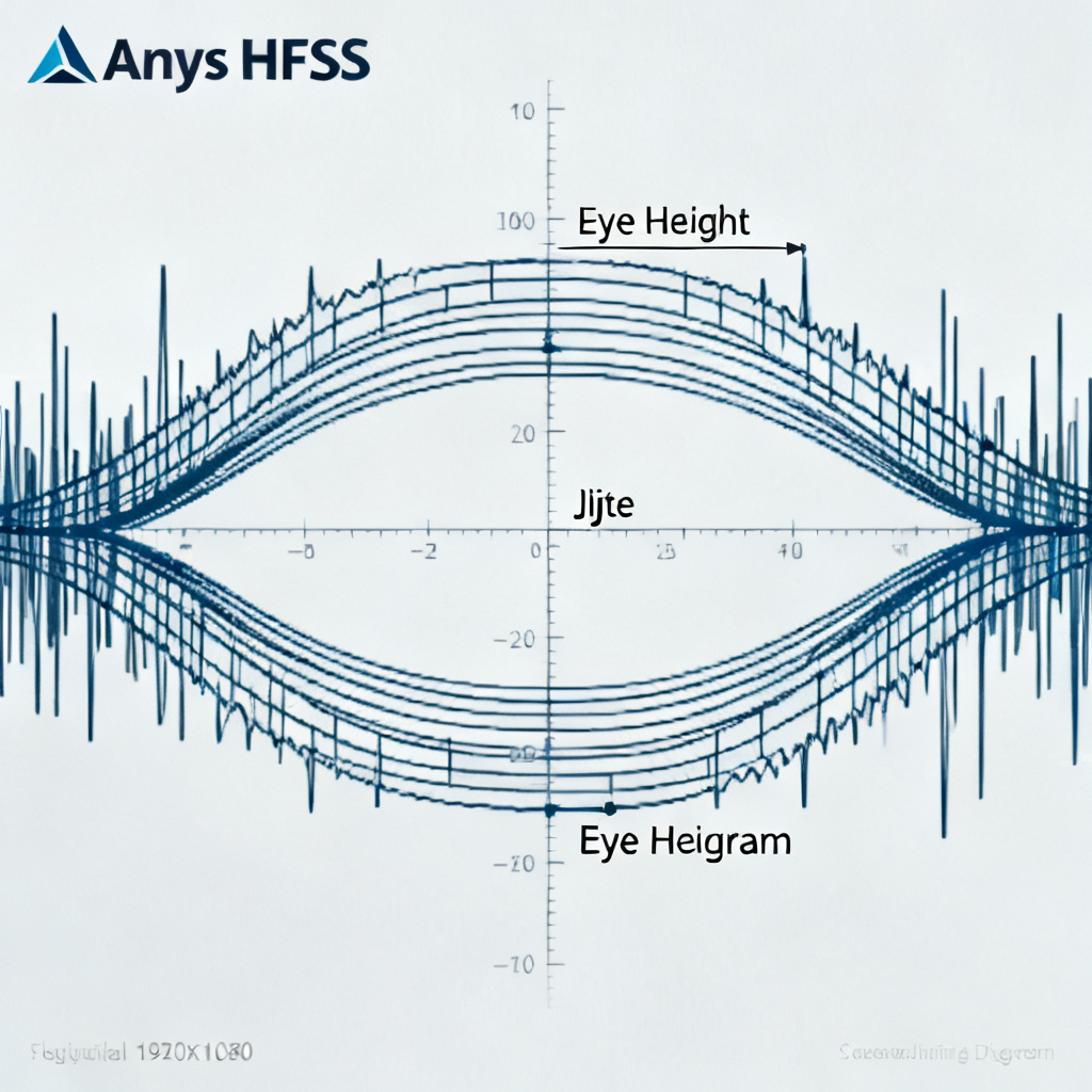
4. View Results: Go to Results > Eye Diagram. HFSS will display the statistical overlay of all bit transitions. You will see:
   • Eye Height: The vertical opening (voltage margin).
   • Eye Width: The horizontal opening (time margin).
   • Jitter: The horizontal spread at the crossing points.
   • Noise: The vertical spread at the center of the eye.

Interpreting Your Results and Optimizing Your PCB

An eye diagram is not an endpoint; it is a diagnostic tool. Here is how to read the results and drive design changes.

Key Metrics to Evaluate

Metric	Definition	Target (Typical High-Speed)
Eye Height	Voltage difference between logic 1 and 0 at the sampling point.	> 200 mV (for 1V logic)
Eye Width	Time window where the signal is stable.	> 70% of the Unit Interval (UI)
Jitter (Pk-Pk)	Total variation in timing of signal edges.	< 20% of UI
Rise/Fall Time	Time for signal to transition between levels.	Matches driver specifications

Common Issues and Fixes

1. Closed Eye (High Loss):
   • Cause: Too much insertion loss (S21) or dielectric loss.
   • Fix: Use lower-loss materials (e.g., Rogers 4350B instead of standard FR4). Increase trace width. Use a shorter trace route. Add a pre-emphasis or equalization circuit in the schematic.
2. Excessive Jitter (Timing Closure):
   • Cause: Impedance discontinuities (vias, connectors) causing reflections.
   • Fix: Back-drill unused via stubs. Optimize via anti-pad size. Ensure 50-ohm (or 100-ohm diff) impedance is maintained throughout the path.
3. Asymmetric Eye (Duty Cycle Distortion):
   • Cause: Skew between differential pair traces.
   • Fix: Use length-matching (trombone or serpentine) to ensure both traces have equal electrical length.

Advanced Optimization

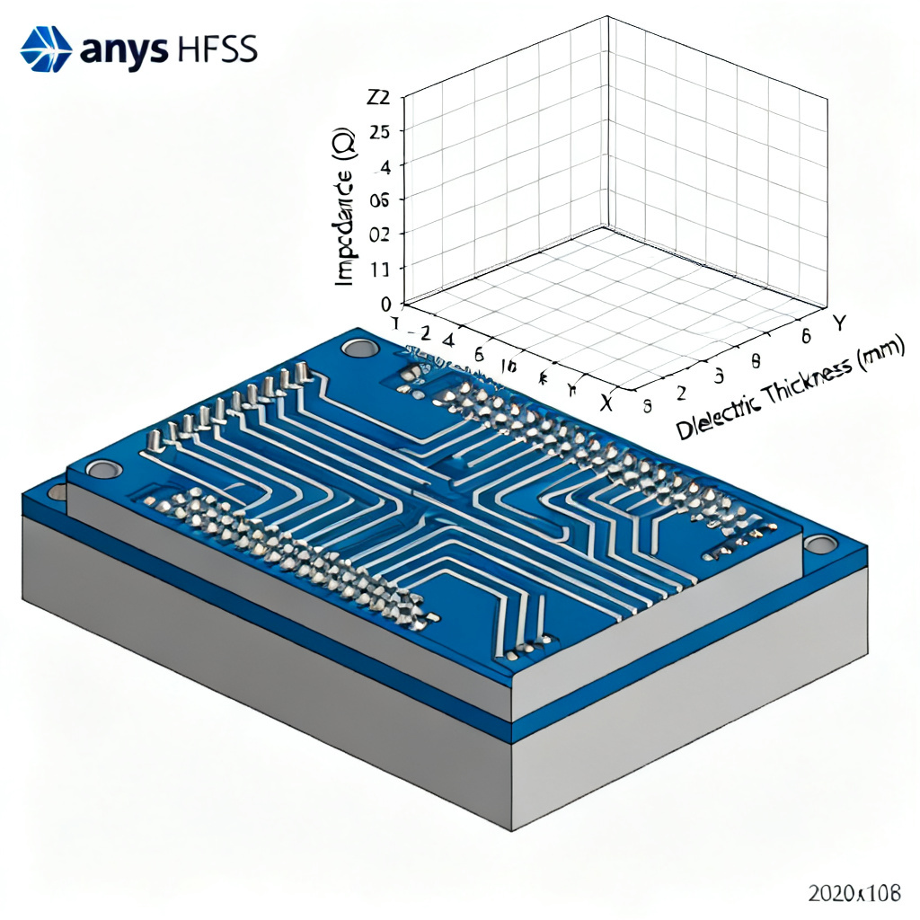
• Parametric Sweep in HFSS: Before finalizing, run a parametric sweep on key variables (e.g., trace width, dielectric thickness, via pad diameter). Re-run the eye diagram for each iteration. This is the most rigorous way to ensure your PCB is ready for fabrication.

Best Practices for B2B High-Speed PCB Designers

To ensure your simulations translate into reliable production PCBs, follow these professional guidelines:

1. Start Simple, Add Complexity: Begin with a single differential pair. Validate your methodology. Then, add crosstalk aggressors, power delivery network (PDN) effects, and multiple layers.
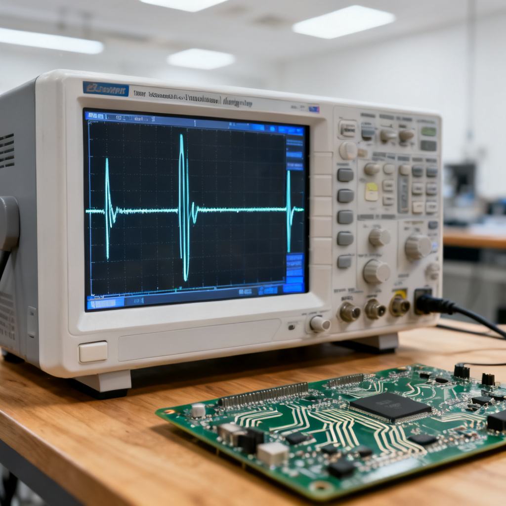
2. Validate with Measurements: Whenever possible, compare your simulated eye diagram against a real oscilloscope measurement (e.g., from a TDR or sampling scope). Calibrate your material models based on empirical data.
3. Use a Consistent Workflow: Save your HFSS project templates with pre-configured materials, ports, and solver settings. This eliminates human error across different design projects.
4. Document Assumptions: Always note the temperature, dielectric model (e.g., Djordjevic-Sarkar for FR4), and mesh convergence criteria in your simulation report. Your client or manufacturing partner will need this for trust.

Frequently Asked Questions

What is an Ansys HFSS eye diagram PCB simulation?

An Ansys HFSS eye diagram PCB simulation is a process that uses the full-wave 3D EM solver to extract S-parameters from a PCB interconnect, then convolves them with a digital stimulus in a circuit simulator to generate an eye diagram. This visual tool helps engineers assess signal integrity by showing voltage margin, timing margin, jitter, and noise in high-speed PCB designs.

How long does an Ansys HFSS eye diagram PCB simulation take?

The duration of an Ansys HFSS eye diagram PCB simulation varies based on model complexity, mesh density, and frequency sweep range. A simple differential pair may take minutes, while a complex multi-layer PCB with multiple vias and connectors can take several hours. Using the Interpolating solver and adaptive mesh refinement can optimize simulation time.

What are common mistakes in Ansys HFSS eye diagram PCB simulation?

Common mistakes in Ansys HFSS eye diagram PCB simulation include using a coarse mesh on critical structures like vias, failing to de-embed ports, choosing an incorrect port type (lumped vs. wave), and not setting the frequency sweep high enough (at least 3-5 times the signal clock rate). These errors can lead to false eye closure or inaccurate jitter measurements.

How do I improve eye diagram results in HFSS?

To improve results in an Ansys HFSS eye diagram PCB simulation, use lower-loss dielectric materials, optimize via design by back-drilling stubs, ensure impedance matching throughout the channel, and run parametric sweeps on trace width and dielectric thickness. Adding equalization in the circuit simulation can also help open the eye.

Conclusion

Generating an eye diagram in Ansys HFSS is a multi-step process that demands precision, but it is the gold standard for validating high-speed PCB designs. By following the combined wisdom of the top experts—from proper port de-embedding to transient analysis configuration—you can confidently predict the performance of your 25 Gbps, 56 Gbps, or even 112 Gbps designs.

At [Your Company Name], we leverage these exact techniques to manufacture high-speed PCBs that perform exactly as simulated. Contact us today for a design review or to request a free simulation analysis for your next project.

Internal Links:

• High-Speed PCB Material Selection Guide
• How to Optimize Via Design for 25 Gbps Signals
• Signal Integrity Testing Services for Prototype PCBs

External References:

• Ansys HFSS User Manual (2024 R2)
• IEEE P802.3bj (100GBASE-KR4) Standards for Eye Mask Requirements