In high-speed PCB design, predicting total jitter and bathtub curve in high speed PCB is essential for ensuring a reliable bit error rate (BER). This guide provides a complete framework for mastering these critical signal integrity concepts.
1. Deconstructing Jitter: The Root Cause of Bit Errors in Total Jitter and Bathtub Curve in High Speed PCB
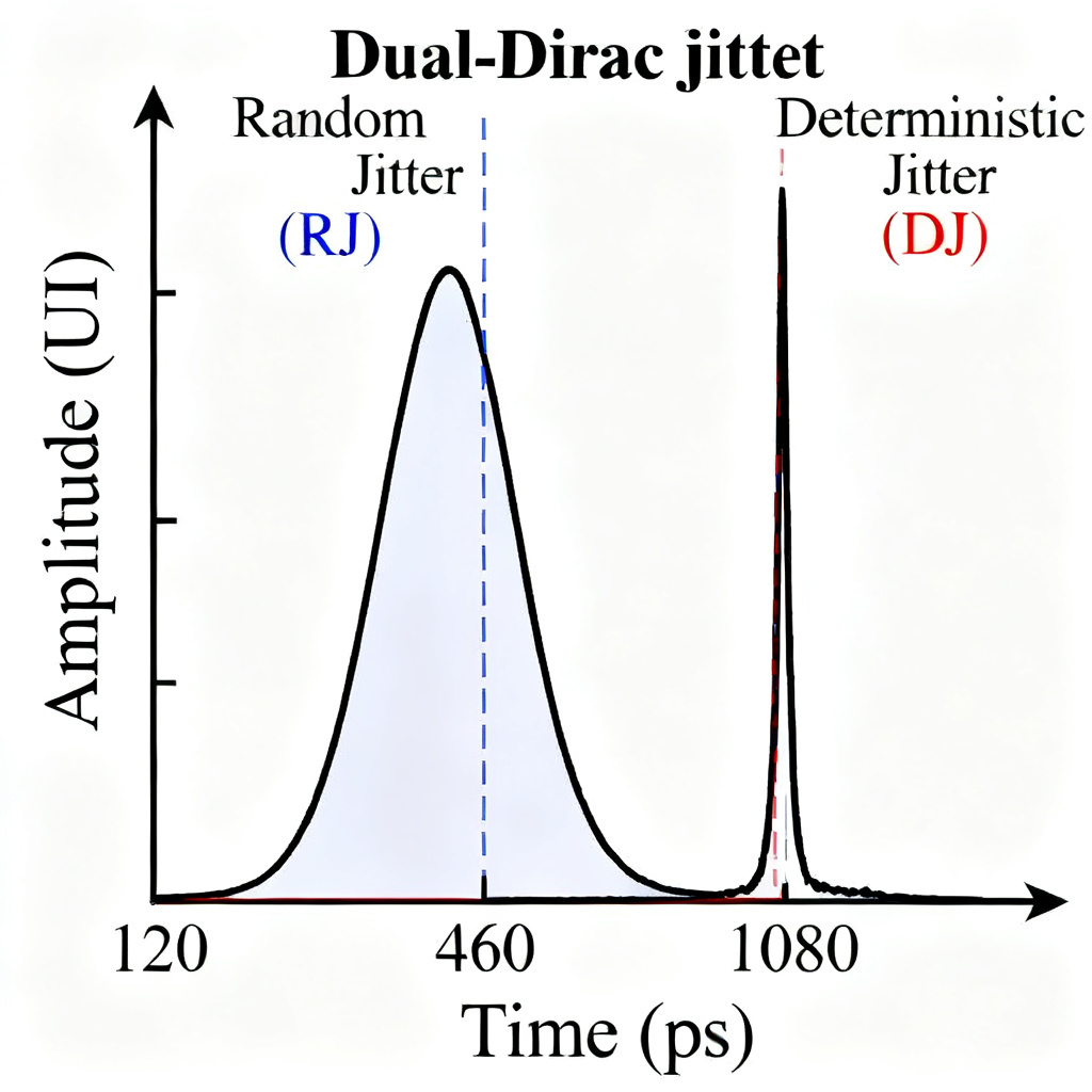
Jitter is the deviation of a signal’s significant instants from their ideal positions in time. It is the primary cause of bit errors in high-speed serial links. To predict BER using total jitter and bathtub curve in high speed PCB, we must first understand jitter’s composition into Random Jitter (RJ) and Deterministic Jitter (DJ).
1.1 Random Jitter (RJ): The Unpredictable Component
Nature: Unbounded, Gaussian, and random. It has no deterministic pattern and is caused by fundamental physical processes like thermal noise, shot noise, and flicker noise in semiconductors and the PCB substrate.
Characteristics:
- Gaussian Distribution: RJ follows a normal probability density function (PDF). Its amplitude is theoretically infinite, but the probability of large jitter values decreases exponentially.
- RMS Value: RJ is typically characterized by its RMS value, often denoted as σ (sigma).
- Peak-to-Peak is Meaningless: Because it is unbounded, the peak-to-peak value of RJ depends entirely on the measurement time.
Impact on BER: RJ is the reason why BER is a probability, not a certainty. Even in a perfectly designed channel, RJ ensures there is always a tiny, non-zero chance of a bit error.
1.2 Deterministic Jitter (DJ): The Predictable Component
Nature: Bounded and predictable. It has a known cause and a finite peak-to-peak amplitude (DJ_pp). DJ is further broken down into sub-components:
- Periodic Jitter (PJ): Correlated to a periodic source like a switching power supply, a clock feedthrough, or a crosstalk aggressor.
- Data-Dependent Jitter (DDJ): Correlated to the specific bit pattern being transmitted. This includes Intersymbol Interference (ISI) and Duty Cycle Distortion (DCD).
Characteristics: The PDF of DJ is often represented by a dual-Dirac or rectangular distribution. Its peak-to-peak value (DJ_pp) is finite and measurable. For modeling purposes, DJ is often simplified to two Dirac delta functions separated by a distance equal to DJ_pp.
1.3 Total Jitter (TJ) – The Sum of All Fears
Total Jitter (TJ) is the peak-to-peak jitter at a specific, very low BER (e.g., 10^-12). It is not simply RJ_pp + DJ_pp. The industry-standard formula for estimating TJ at a target BER is the Dual-Dirac Model: TJ(BER) = DJ_pp + 2 × α × RJ_rms.
Where DJ_pp is the peak-to-peak deterministic jitter, RJ_rms is the RMS value of the random jitter, and α is a constant derived from the inverse of the Q-function. For a BER of 10^-12, α ≈ 7.0. For 10^-15, α ≈ 7.9.
Critical Insight: This formula illustrates a key trade-off. A small increase in RJ_rms can dramatically increase TJ at a low BER, while a large DJ_pp directly adds to the bottom line. Reducing DJ is the most effective way to improve BER.
2. The Bathtub Curve – A Visual BER Predictor for Total Jitter and Bathtub Curve in High Speed PCB
The bathtub curve is a graphical representation of a system’s BER as a function of the sampling point within a Unit Interval (UI). It is the most intuitive way to visualize the relationship between jitter and BER.
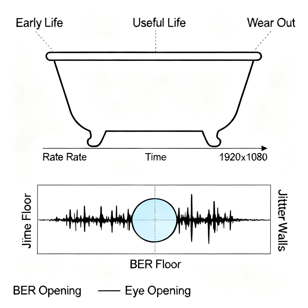
2.1 Anatomy of the Bathtub Curve
Imagine a single bit period (1 UI). The receiver must sample the incoming data at a precise moment to determine if it’s a ‘1’ or a ‘0’. The bathtub curve plots the BER on the y-axis (log scale) against the sampling position (from 0 to 1 UI) on the x-axis.
- The Walls: The left wall represents the probability of a bit error when sampling near the rising edge; the right wall represents the same near the falling edge.
- The Flat Bottom: The region in the center of the UI where the BER is at its minimum (ideally zero, but in practice, the BER floor).
- The Eye Opening: The horizontal opening of the eye at a specific BER target.
2.2 How to Read and Interpret the Curve
1. Identify the Target BER: Draw a horizontal line at your target BER (e.g., 10^-12). 2. Find the Eye Opening: The distance between the left and right walls at this BER line is the eye opening. 3. Calculate Total Jitter (TJ): Total Jitter is the complement of the eye opening. TJ = 1 UI – Eye Opening. 4. Assess Margin: The wider the eye opening at your target BER, the more margin you have.
- Steep Walls (DJ Dominant): The bathtub curve has very steep, almost vertical walls, and a wide, flat bottom. This indicates that Deterministic Jitter (DJ) is the dominant source.
- Gradual, Curved Walls (RJ Dominant): The walls of the bathtub curve are gently sloped, curving outwards. This indicates that Random Jitter (RJ) is the dominant source.
2.3 The BER Floor: The Limit of Your Design
The BER floor is the flat, minimum BER value in the center of the bathtub curve. In an ideal system, this would be 0. In reality, it is a non-zero value caused by residual DJ, clock recovery issues, and non-linearities. A high BER floor means that even with perfect sampling, you will still have a certain number of errors.
3. From Theory to Practice – Predicting BER in Your PCB Design Using Total Jitter and Bathtub Curve in High Speed PCB
Now that you understand the theory, how do you actually use these concepts to predict BER for your specific PCB design?
3.1 Step-by-Step Simulation Workflow
Before you build a prototype, you can predict BER with high accuracy using modern EDA tools.
- Extract Channel Model (S-parameters): Simulate your PCB trace, vias, connectors, and package models to get the S-parameter model.
- Create a Transient Simulation: Use a circuit simulator to drive your channel model with a pseudo-random bit sequence (PRBS) pattern.
- Build a Jitter Histogram: At the receiver’s sampling point, the simulator accumulates timing errors for every bit edge.
- Separate RJ and DJ: The simulator uses statistical algorithms to decompose the histogram into its RJ and DJ components.
- Plot the Bathtub Curve: The simulator extrapolates the histogram’s tails to the target BER using the Dual-Dirac model.
- Extract TJ and Eye Opening: From the curve, you can directly read the eye opening and the Total Jitter at your target BER.
3.2 The Q-Factor and the Q-Scale Method
The Q-factor is a dimensionless parameter that converts a BER requirement into a “number of sigmas” of Gaussian jitter. The relationship is: BER = 1/2 × erfc(Q/√2). For BER = 10^-12, Q = 7.0. For BER = 10^-15, Q = 7.9.
The Q-Scale Method is a powerful graphical technique used in oscilloscopes and simulation tools. Instead of plotting BER on a linear or log scale, it plots the inverse of the Q-function on the y-axis. This transforms the bathtub curve into straight lines.
On a Q-scale plot, the slope of the lines is directly proportional to the RMS value of the Random Jitter (RJ_rms). The separation between the lines at the top is the Deterministic Jitter (DJ_pp). You can then predict TJ at any BER by using the formula: TJ = DJ_pp + 2 × Q(BER) × RJ_rms.
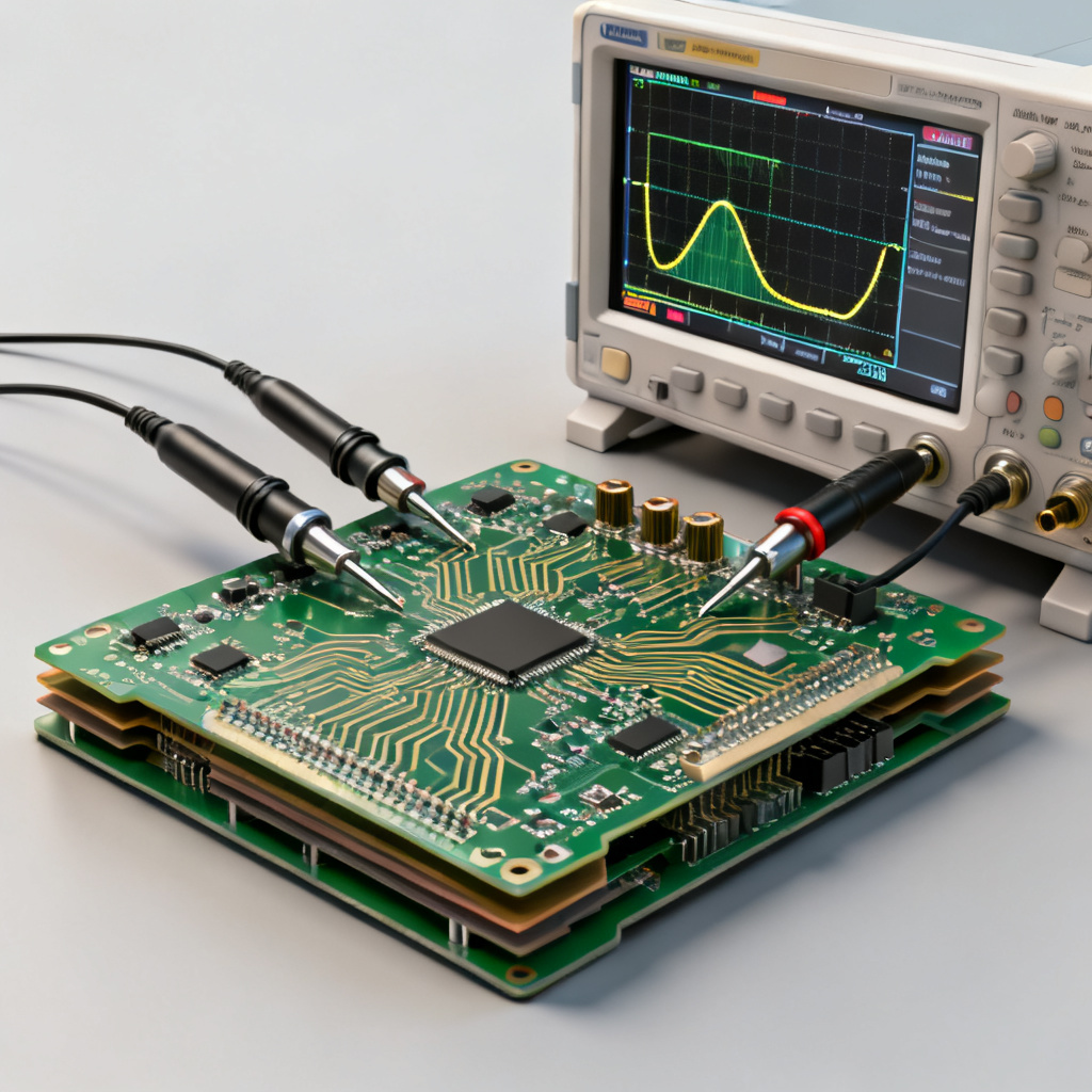
3.3 Measurement and Compliance Testing
In the lab, a Real-Time Oscilloscope (RTO) or a Sampling Oscilloscope with jitter analysis software is used to perform these predictions. Eye diagrams, BER contour plots, and compliance tests for standards like PCIe, USB, and Ethernet all rely on total jitter and bathtub curve in high speed PCB analysis.
4. Practical Design Guidelines to Minimize Jitter for Total Jitter and Bathtub Curve in High Speed PCB
Understanding jitter is useless without knowing how to fight it. Here are actionable strategies for your high-speed PCB layout.
4.1 Combat ISI (The Biggest DJ Culprit)
- Use Low-Loss Materials: For high-speed traces, use materials like Megtron 6, Rogers, or Isola.
- Minimize Trace Length: Every inch of trace adds loss and delay.
- Match Impedance Rigorously: Any impedance discontinuity creates reflections that cause ISI.
- Use Pre-Emphasis and Equalization: Most modern transceivers have built-in equalizers (CTLE, DFE) and pre-emphasis/de-emphasis.
4.2 Minimize Crosstalk (PJ and DJ)
- Increase Spacing: The 3-W or 5-W rule (spacing traces 3-5 times the trace width apart) is a good starting point.
- Use Ground Planes: A solid ground plane adjacent to the signal layer acts as a shield.
- Route Differential Pairs Tightly: For high-speed differential signals, route the positive and negative traces close together.
4.3 Clean Up the Power Supply (PJ)
- Proper Decoupling: Use a combination of bulk, ceramic, and low-ESR capacitors near the power pins.
- Use Dedicated Power Planes: A clean, low-inductance power plane is essential.
- Isolate Analog and Digital Sections: Keep the power supplies for high-speed analog circuits separate from noisy digital supplies.
4.4 Control DCD (Duty Cycle Distortion)
- Match Rising and Falling Edge Delays: Ensure that the driver and receiver have symmetric rise and fall times.
- Avoid AC-Coupling on Clock Lines: AC-coupling capacitors can introduce DCD if not properly chosen.
Comparison Table: Key Parameters in Total Jitter and Bathtub Curve in High Speed PCB
| Parameter | Description | Impact on Total Jitter |
|---|---|---|
| Random Jitter (RJ_rms) | Gaussian noise from thermal and shot noise | Increases exponentially at low BER |
| Deterministic Jitter (DJ_pp) | Bounded jitter from ISI, crosstalk, DCD | Adds directly to TJ |
| Q-Factor | Converts BER to sigma units | Q=7.0 for BER=10^-12 |
| Eye Opening | Horizontal sampling window | Inversely proportional to TJ |
| BER Floor | Minimum achievable BER | Limits system performance |
FAQ: Total Jitter and Bathtub Curve in High Speed PCB
What is total jitter and bathtub curve in high speed PCB?
Total jitter and bathtub curve in high speed PCB are critical metrics for predicting the bit error rate (BER) of a high-speed digital channel. Total jitter combines random and deterministic components, while the bathtub curve visualizes BER as a function of sampling position.
How do I predict BER using total jitter and bathtub curve in high speed PCB?
To predict BER, you decompose jitter into RJ and DJ using the Dual-Dirac model, then plot the bathtub curve. The eye opening at your target BER directly gives the system margin.
What is the difference between RJ and DJ in total jitter analysis?
Random Jitter (RJ) is unbounded and Gaussian, while Deterministic Jitter (DJ) is bounded and predictable. In total jitter and bathtub curve in high speed PCB, DJ dominates the steepness of the bathtub walls, while RJ determines the curvature.
How can I reduce total jitter in my high-speed PCB design?
Reduce total jitter by using low-loss materials, matching impedance, minimizing crosstalk, cleaning up power supplies, and controlling duty cycle distortion. These techniques directly improve the bathtub curve and lower BER.