Master the bathtub curve extrapolation method for predicting jitter in high-speed PCBs at low BER. This guide explains how to analyze deterministic and random jitter, apply statistical models, and ensure signal integrity for reliable data transmission.
1. Understanding Jitter and BER Fundamentals
1.1 What Is Jitter in High-Speed PCBs?
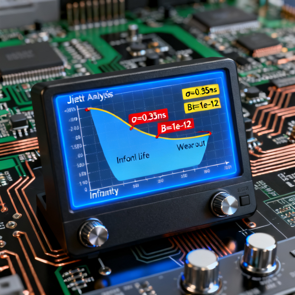
Jitter in high-speed PCB design is the time-domain variation of signal edges from ideal positions. It causes data errors by shifting sampling points. Jitter is categorized as random jitter (RJ)—Gaussian, unbounded, from thermal noise—and deterministic jitter (DJ)—bounded, from data patterns or system imperfections like intersymbol interference (ISI), periodic jitter (PJ), or duty-cycle distortion (DCD).
1.2 Bit Error Rate (BER) and Its Importance
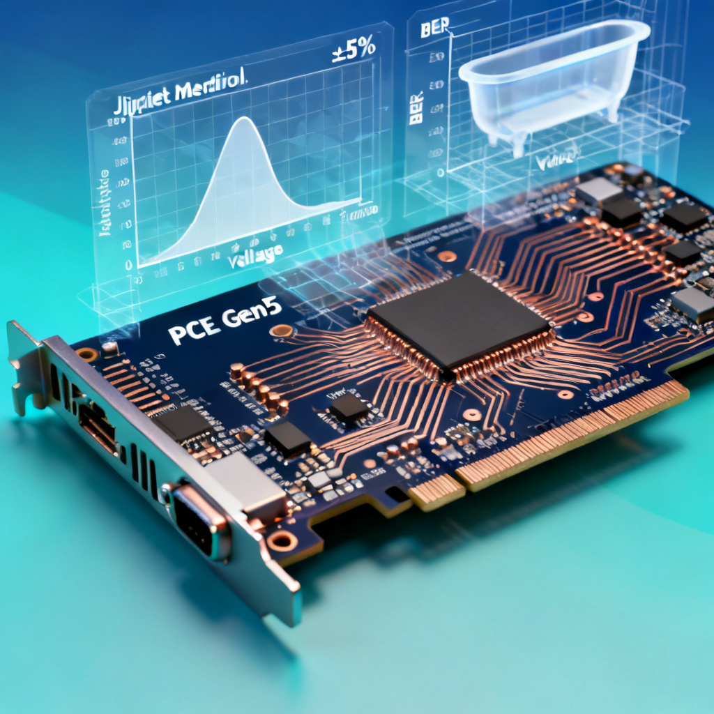
BER is the ratio of erroneous bits to total transmitted bits. For high-speed PCBs, acceptable BER is 10⁻¹² or lower. The bathtub curve visualizes how BER varies with sampling phase, showing the “eye” opening where BER is minimal.
1.3 The Bathtub Curve as a Visual Tool
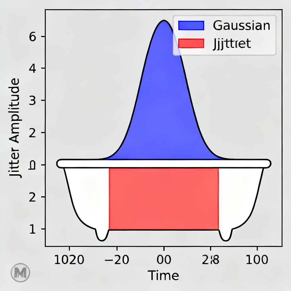
The bathtub curve plots BER on a logarithmic scale against sampling phase. It has three regions: left tail (BER increases near left data edge), right tail (BER increases near right data edge), and flat bottom (optimal sampling region). The shape is dominated by DJ in tails and RJ in the flat region. Extrapolation leverages RJ’s Gaussian nature to predict jitter at extreme phases.
2. Bathtub Curve Extrapolation Methodology
2.1 Why Extrapolate? The Challenge of Low BER Measurement
Measuring BER at 10⁻¹² directly requires trillions of bits—time-prohibitive for high-speed links. At 10 Gbps, measuring 10⁻¹² BER takes minutes, but 10⁻¹⁵ takes hours. Bathtub curve extrapolation estimates jitter at low BER using faster statistical techniques.
2.2 The Dual-Dirac Model
The Dual-Dirac model assumes jitter consists of bounded DJ (two Dirac delta functions) and Gaussian RJ. Total jitter (TJ) at a given BER is: TJ(BER) = DJ + 2 × α × RJ, where α is from the inverse Q-function (e.g., α ≈ 7.034 for BER=10⁻¹²). This linearizes the bathtub curve on a Q-scale plot.
2.3 Step-by-Step Extrapolation Process
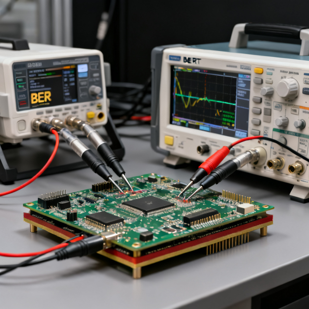
Step 1: Measure jitter components using a high-bandwidth oscilloscope or BERT. Extract RJ (RMS) and DJ (peak-to-peak) via tail-fit methods. Step 2: Plot the bathtub curve by measuring BER at multiple sampling phases. Step 3: Fit the Dual-Dirac model by converting BER to Q-scale. Step 4: Extrapolate to target BER using the linear fit. The total jitter is the sum of left and right tail extrapolations.
2.4 Key Considerations for Accurate Extrapolation
Ensure 5–10 measurement points per tail to avoid overfitting. The Dual-Dirac model assumes Gaussian RJ; non-Gaussian noise (e.g., crosstalk) can skew results. DJ must be bounded; unbounded periodic jitter causes underestimation. Use averaging and filtering to reduce system noise.
3. Practical Application in High-Speed PCB Design
3.1 Predicting Jitter for Low BER Compliance
For standards like PCIe Gen 4/5, USB 3.2, and 100GbE, jitter budgets are specified at BER 10⁻¹². Bathtub curve extrapolation enables compliance verification without long-duration testing. For a 28 Gbps NRZ link, measure jitter at BER 10⁻⁶ and extrapolate to 10⁻¹² to check if TJ meets the 0.3 UI budget.
3.2 Optimizing PCB Layout and Material Selection
Extrapolation results guide design decisions: low-loss materials (e.g., Rogers 4350B, Megtron 6) reduce ISI-related DJ, flattening bathtub curve tails. 50‑ohm ±10% impedance control minimizes reflections and DCD. Via stub mitigation (back-drilling or blind vias) reduces resonant peaks that add PJ.
3.3 Case Study: 25 Gbps Backplane Design
A backplane with FR4 shows DJ of 15 ps and RJ of 1.5 ps RMS. Using the Dual-Dirac model, at BER 10⁻¹², TJ = 15 + 2×7.034×1.5 ≈ 36.1 ps. The eye opening at 40 ps UI (25 Gbps) is only 3.9 ps—marginal. Switching to low-loss material reduces DJ to 10 ps and RJ to 1.0 ps RMS, yielding TJ = 24.1 ps and a comfortable 15.9 ps eye opening.
3.4 Tools and Software for Extrapolation
Keysight ADS includes bathtub curve simulation with statistical eye diagrams. Ansys HFSS handles channel modeling and jitter extraction. Teledyne LeCroy SDA offers automated Dual-Dirac fitting. Open-source Python scripts use scipy for Q-scale fitting.
4. Advanced Topics and Limitations
4.1 Extending Beyond the Dual-Dirac Model
For non-Gaussian RJ (e.g., clock jitter), the Dual-Dirac model may underestimate TJ. Advanced models include gamma distribution fit for skewed histograms and convolution-based methods that numerically convolve RJ and DJ distributions to predict BER.
4.2 Impact of Equalization
Equalization techniques (CTLE, DFE, FFE) reduce DJ by compensating for channel loss but amplify noise, affecting RJ. Jitter in high-speed PCB analysis must account for equalizer responses, often requiring post-equalization jitter analysis.
4.3 Limitations and Pitfalls
Extrapolation beyond measured data increases uncertainty—for BER 10⁻¹⁵, errors can exceed 20%. Oscilloscope bandwidth and sampling rate limit high-frequency jitter capture. Temperature and voltage variations require derating factors.
4.4 Future Trends: Machine Learning for Jitter Prediction
Emerging neural network techniques predict bathtub curves from channel S-parameters, reducing measurement time. However, these are not yet standardized for compliance testing.
5. Best Practices for B2B PCB Manufacturing and Export
5.1 Communicating Jitter Specifications to Clients
When quoting high-speed PCB designs, include jitter budget analysis in the SI report. Example: “Based on bathtub curve extrapolation, our 12-layer stackup with Megtron 6 yields TJ < 20 ps at BER 10⁻¹² for 10 Gbps links.”
5.2 Ensuring Repeatability and Reliability
Use consistent measurement setups (same oscilloscope model, probes). Perform statistical process control (SPC) on dielectric constant and copper roughness.
5.3 Leveraging Content for SEO and Trust
This pillar content demonstrates expertise in advanced signal integrity, attracting engineers searching for “bathtub curve jitter prediction” or “high-speed PCB BER analysis.” Link from product pages for 10+ layer boards and high-frequency laminates.
FAQ
What is bathtub curve extrapolation in high-speed PCB design?
Bathtub curve extrapolation is a statistical method used to predict jitter at low BER (e.g., 10⁻¹²) by extending the tails of the BER vs. sampling phase curve. It relies on the Dual-Dirac model to estimate total jitter from random and deterministic components.
How does the Dual-Dirac model help predict jitter?
The Dual-Dirac model separates jitter into Gaussian random jitter and bounded deterministic jitter. By fitting the bathtub curve on a Q-scale, engineers can extrapolate to target BER levels, enabling compliance verification for standards like PCIe 5.0.
What tools are used for bathtub curve extrapolation?
Common tools include Keysight ADS, Ansys HFSS, Teledyne LeCroy SDA, and Python scripts with scipy. These support measurement, fitting, and extrapolation for jitter in high-speed PCB analysis.
Why is low BER important for high-speed PCBs?
Low BER (e.g., 10⁻¹²) ensures data integrity in high-speed serial links. Without accurate jitter prediction, systems may experience errors in critical applications like data centers or telecommunications.
Conclusion
Bathtub curve extrapolation via the Dual-Dirac model is a proven method for predicting jitter at low BER in high-speed PCBs. By understanding RJ and DJ interactions, engineers validate compliance, optimize designs, and reduce time-to-market. Despite limitations, combining this technique with proper measurement practices and advanced materials ensures reliable data transmission. For B2B PCB manufacturers, mastering this methodology is a competitive advantage for serving clients in telecommunications, data centers, and aerospace.