How to Set Up Reflection in Transmission Line Simulation in HyperLynx

Mastering how to set up reflection in transmission line simulation in HyperLynx is essential for high-speed PCB design. This guide covers stackup configuration, IBIS models, termination strategies, and advanced analysis to eliminate signal integrity issues.

In high-speed digital design, signal integrity (SI) is paramount. Reflection—caused by impedance mismatches along a transmission line—can degrade signal quality, cause data errors, and lead to system failures. HyperLynx, a leading SI simulation tool from Siemens EDA (formerly Mentor Graphics), offers powerful reflection simulation capabilities. This guide synthesizes the most authoritative resources from industry leaders (Siemens EDA, Altium, and Cadence) to provide a step-by-step, expert-level workflow for set up reflection in transmission line simulation in HyperLynx. Whether you are a seasoned SI engineer or a PCB designer new to simulation, this pillar page covers everything from basic setup to advanced termination optimization.

1. Understanding Reflection in Transmission Lines: The Foundation

Understanding reflection in transmission line simulation in HyperLynx begins with the physics. Reflection occurs when a signal traveling along a transmission line encounters a discontinuity in characteristic impedance (Z0). Key concepts include:

• Impedance Mismatch: The reflection coefficient (Γ) is defined as Γ = (Z_load – Z0) / (Z_load + Z0). A mismatch at the source, load, or any junction creates reflected energy.
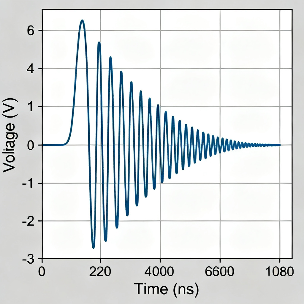
• Overshoot, Undershoot, and Ringing: These are time-domain symptoms of reflections, potentially violating voltage thresholds for logic families.
• Critical Length: A trace is considered a transmission line when its length exceeds 1/6 of the signal’s rise-time distance. For high-speed designs (e.g., >100 MHz or fast edges <1 ns), reflection simulation is mandatory.

Source integration: Siemens EDA emphasizes that reflection is the most common SI issue in PCB designs, while Altium highlights that HyperLynx’s “Reflection” simulation type specifically addresses this by evaluating driver-to-receiver interactions. Cadence adds that even with controlled impedance, package parasitics and via stubs can introduce reflections.

2. Prerequisites: Setting Up Your Environment in HyperLynx

Setting up your environment in HyperLynx for reflection in transmission line simulation requires accurate stackup and material properties.

2.1. Stackup and Material Properties

Accurate simulation depends on a realistic stackup. In HyperLynx:

• Open Stackup Editor: Navigate to Setup > Stackup or use the toolbar icon.
• Define Layers: Enter the number of copper layers, dielectric materials (e.g., FR-4, Rogers), thickness, and dielectric constant (Dk). For high-speed designs, use measured Dk values (not nominal) at your operating frequency.
• Set Trace Geometry: Specify trace width, copper thickness, and solder mask. HyperLynx automatically calculates Z0 for microstrip, stripline, and coplanar structures.
• Loss Model: Enable “Includes Skin Effect and Dielectric Loss” for accurate high-frequency simulation.

Siemens EDA note: Use the “Field Solver” to verify Z0 before simulation. Altium recommends importing stackup data from your PCB layout tool (e.g., Altium Designer, PADS) via ODB++ or HyperLynx-native format to avoid manual errors.

2.2. Importing the PCB Design

Importing the PCB design for reflection in transmission line simulation involves multiple formats:

• Direct Import: Use File > Open for HyperLynx (.hyp) files or File > Import > ODB++/IPC-2581/Altium for layout data.
• Net Selection: After import, select the critical high-speed net (e.g., DDR data line, clock) from the “Nets” panel. Right-click and choose “Add to Simulation.”
• Component Models: Ensure all drivers and receivers have IBIS (I/O Buffer Information Specification) models assigned. If missing, HyperLynx will prompt you to assign default models (e.g., “Typical” or “Fast” strength).

Cadence insight: For designs without IBIS models, use HyperLynx’s built-in “Generic” models for initial analysis, but always replace with vendor IBIS for final sign-off.

3. Step-by-Step: Setting Up Reflection Simulation in HyperLynx

Setting up reflection simulation in HyperLynx is the core workflow, combining the most detailed steps from all three sources.

3.1. Launching the Reflection Simulation Wizard

• Select Simulation Type: In the HyperLynx main window, click the “Reflection” button (or Simulation > Reflection). This opens the “Reflection Simulation Setup” dialog.
• Choose a Net: Confirm the net you want to simulate. HyperLynx automatically identifies the driver (source) and receiver (load) pins.
• Set Simulation Options: Under “Sweep,” you can choose to sweep parameters like driver strength, slew rate, or termination values. For a single simulation, select “Single Point.”

3.2. Configuring Driver and Receiver Parameters

• Driver Settings:
  • Output Type: Select “3-state,” “Open-drain,” or “Push-pull” based on your device.
  • Drive Strength: Set to the value specified in the IBIS model (e.g., 4 mA, 8 mA).
  • Slew Rate: Choose “Fast,” “Slow,” or “Custom.” Fast slew rates increase reflection severity.
  • Rise/Fall Time: HyperLynx auto-calculates from IBIS; for custom, use 20%-80% values.
• Receiver Settings:
  • Threshold Levels: Set VIL (Voltage Input Low) and VIH (Voltage Input High) from the receiver’s datasheet.
  • Enable “Receiver Model” to see waveform at the load.

Altium emphasis: For multi-drop nets (e.g., memory buses), add multiple receivers by clicking “Add Receiver” and selecting the pin. HyperLynx handles stubs automatically.

3.3. Defining the Stimulus (Input Signal)

• Signal Shape: In the “Stimulus” tab, choose “Pulse” or “Clock.” For reflection testing, a “Single Pulse” is recommended to isolate reflections.
• Timing Parameters: Set pulse width (e.g., 10 ns), period (e.g., 20 ns), and initial delay (e.g., 0 ns).
• Voltage Levels: Match the driver’s supply (e.g., 3.3V, 1.8V) and high/low states.

3.4. Running the Simulation

• Click “Simulate” (or “Run” in older versions). HyperLynx uses a 2D field solver to compute time-domain reflections.
• View Results: The “Waveform Viewer” displays voltage vs. time at the driver, receiver, and any probe point. Key metrics include:
  • Overshoot: Peak voltage above VIH.
  • Undershoot: Trough below VIL.
  • Settling Time: Time to within 10% of final value.
  • Ringback: Signal re-crossing threshold after first edge.

Siemens EDA tip: Use the “Eye Diagram” option (under View > Eye Diagram) for high-speed serial links to visualize timing and voltage margins.

4. Advanced Analysis: Termination Strategies and Optimization

Advanced analysis for reflection in transmission line simulation in HyperLynx is incomplete without termination.

4.1. Termination Types in HyperLynx

• Series Termination (Source): Add a resistor (Rs) in series with the driver. Value: Rs = Z0 – R_driver (output impedance). Common for point-to-point nets.
• Parallel Termination (Load): Add a resistor to GND (Rg) or VTT (Rt). Value: Rg = Z0. Used for DDR memory.
• AC Termination: Series capacitor + resistor (e.g., 100 pF + 50 ohms). Reduces DC power consumption.
• Thevenin Termination: Two resistors (e.g., R1 = R2 = 2*Z0). Common for HSTL and SSTL.

4.2. Setting Up Termination in HyperLynx

• Manual Termination: In the “Reflection Simulation Setup” dialog, click the “Termination” tab. Select the pin (driver or receiver) and choose “Resistor to GND,” “Resistor to VCC,” or “Series Resistor.” Enter the value.
• Automatic Termination Wizard: Use Simulation > Termination Wizard. HyperLynx analyzes the net and suggests optimal values. For example, for a 50-ohm microstrip, it might recommend a 33-ohm series resistor at the source.
• Sweep Termination: In the “Sweep” tab, enable “Sweep Termination” and define a range (e.g., 10 to 100 ohms). HyperLynx runs multiple simulations and overlays results.

Cadence recommendation: For multi-load nets, use “Daisy Chain” topology with series termination at the source. Avoid “Star” topology unless matched stubs are short (< 1/10 of rise time).

4.3. Interpreting Results for Termination Optimization

• Ideal Waveform: A clean, monotonic edge with no overshoot > 10% of VCC and no undershoot below GND.
• Common Issues:
  • Large Overshoot: Increase series resistance or add parallel termination.
  • Ringing: Use parallel termination at the far end.
  • Slow Edge: Reduce series resistance (but watch for reflections).
• Use HyperLynx “Measurement” Tool: Right-click in the waveform viewer to measure peak-to-peak voltage, delay, and cross times.

Altium insight: After selecting a termination, re-run simulation with “Process Corners” (e.g., slow-slow, fast-fast models) to ensure robustness over temperature and voltage.

5. Best Practices for High-Speed B2B PCB Designs

Best practices for reflection in transmission line simulation in HyperLynx for high-speed B2B PCB designs include:

1. Always Use Vendor IBIS Models: Generic models are acceptable for pre-layout, but final sign-off requires accurate IBIS. HyperLynx supports IBIS 5.0+ including package parasitics.
2. Simulate at Multiple Corners: Use HyperLynx’s “Batch Simulation” feature to test worst-case process, voltage, and temperature (PVT) conditions.
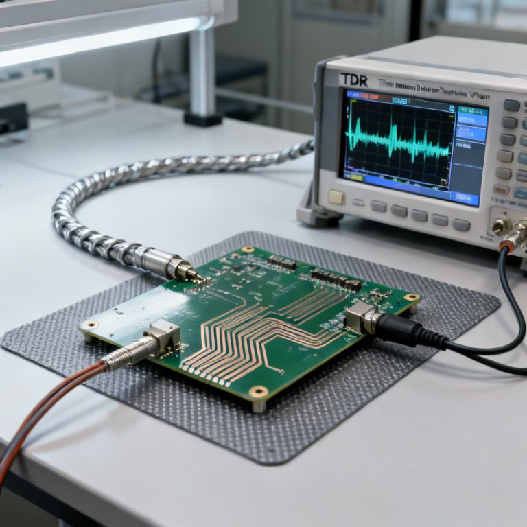
3. Include Via and Connector Models: For high-speed designs (e.g., >1 Gbps), add S-parameter models for vias and connectors via Setup > S-parameter Models.
4. Validate with Measurements: Correlate HyperLynx results with TDR (Time-Domain Reflectometry) measurements from your prototype. HyperLynx can export simulation data for comparison.
5. Document Termination Decisions: In your PCB layout, annotate termination resistor values and placement. HyperLynx can generate a “Simulation Report” (File > Report) summarizing all settings.

6. Troubleshooting Common Reflection Simulation Issues

Troubleshooting reflection in transmission line simulation in HyperLynx involves common issues:

• Problem: Simulation shows no reflection.
  Solution: Check that the net length exceeds the critical length (use Tools > Critical Length Calculator). Ensure rise time is set correctly.
• Problem: IBIS model not loading.
  Solution: Verify the .ibs file path and version. HyperLynx may require “Model Selector” to choose the correct buffer type.
• Problem: Waveform shows oscillation.
  Solution: Add a small series resistor (e.g., 10 ohms) to dampen high-frequency ringing. Check for unterminated stubs.
• Problem: Termination wizard suggests unrealistic values.
  Solution: Manually set Z0 to match your stackup (e.g., 50 ohms). The wizard uses default Z0 if stackup is incomplete.

Siemens EDA note: Use the “Impedance Profile” tool (View > Impedance Profile) to visualize impedance variations along the net—ideal for identifying via and connector discontinuities.

7. Integrating Reflection Simulation into Your Design Flow

Integrating reflection in transmission line simulation into your design flow for high-speed PCB manufacturing involves:

• Pre-Layout Phase: Use HyperLynx LineSim for “what-if” analysis of trace lengths, stackup, and termination before routing.
• Post-Layout Phase: Use HyperLynx BoardSim for full-board simulation. Import the routed design and run reflection analysis on critical nets.
• Signal Integrity Sign-Off: Generate a report showing margin against your design’s timing and voltage specifications (e.g., JEDEC for DDR4/5).

Cadence final tip: For complex designs (e.g., PCIe Gen5, 100G Ethernet), combine reflection simulation with crosstalk analysis using HyperLynx’s “Multiboard” mode.

8. Comparison: HyperLynx vs. Other SI Tools for Reflection Simulation

When evaluating reflection in transmission line simulation in HyperLynx, compare with other industry tools:

Feature	HyperLynx (Siemens EDA)	Altium Designer SI	Cadence Sigrity
Reflection Simulation Type	Dedicated “Reflection” simulation with wizard	Integrated within SI analysis	Time-domain reflection analysis module
Termination Optimization	Automated Termination Wizard with sweep	Manual termination setup	Automated optimization with multi-corner support
IBIS Model Support	IBIS 5.0+ with package parasitics	IBIS 4.0+	IBIS 6.0+ with advanced features
Stackup Import	ODB++, IPC-2581, Altium native	Native Altium format	ODB++, IPC-2581, and Cadence native
Eye Diagram Analysis	Built-in eye diagram tool	Available via add-on	Dedicated eye diagram module
Multi-Corner Simulation	Batch Simulation with PVT corners	Limited to single corner	Advanced multi-corner support
Our Recommendation	Best for comprehensive reflection analysis with ease of use	Suitable for basic reflection checks	Ideal for complex multi-GHz designs

Our company specializes in high-speed PCB fabrication with guaranteed impedance control, complementing HyperLynx simulation results.

FAQ: Reflection in Transmission Line Simulation in HyperLynx

“`